MS Excel - Freeze panes

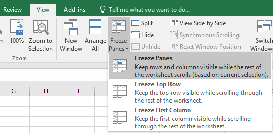
In MS Excel, using Freeze Panes feature on selected columns is tricky. First, you have to select from the right to the left and you have to select 1 extra column from the right. Then, navigate to View > Freeze Panes and select Freeze Panes.

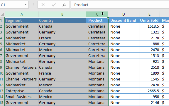
For example, suppose that you have the following data. If you want to freeze columns Segment and Country, then you have to select columns in the following order: Product, Country, Segment. Finally, select the Freeze Panes.

The same principle apply to the rows. Therefore, you have to select from the bottom to the top and you have to select 1 extra row from the bottom.