In MS Excel, you can use the powerful Pivot table to get aggregate information from your data.
Assume that you have the following information. The table below shows the price of each fruit sold per day.
| Date | Fruit | Price |
|---|---|---|
| 2020-01-11 | Banana | 2.99 |
| 2020-01-11 | Orange | 0.99 |
| 2020-01-11 | Banana | 2.99 |
| 2020-02-22 | Strawberries | 1.99 |
| 2020-02-22 | Mango | 3.66 |
| 2020-02-22 | Apple | 4.56 |
Total value sold per fruit
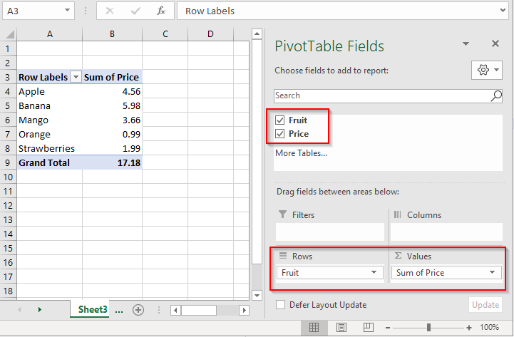
If you want to know how the total value sold per fruit, then you have to group by fruit and sum the prices.
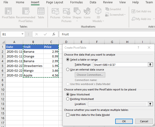
- Select Fruit and Price columns.
- Insert PivotTable.
- Check the Fruit and Price fields. Ensure that the Values field is set to Sum of Price.
Total fruit sold per day
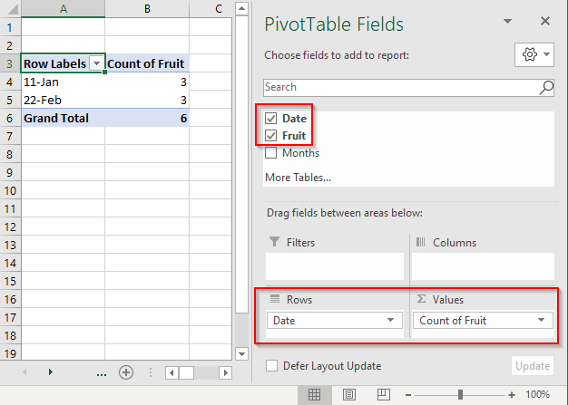
If you want to know how many fruits were sold per day, then you have to group by date and count the instance of fruit.
- Select Date and Fruit columns.
- Insert PivotTable.
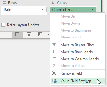
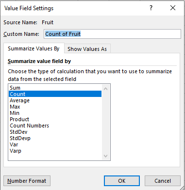
- Check the Date and Fruit fields. Ensure that Date is under Rows and Count of Fruit is under Values.
Other functions
MS Excel offers other aggregate functions too, such as average, maximum, minimum and etc.
